Since ancient times, quantitative methods of planning and decision-making have helped a person. How much grain to plant based on the number of people in the family? What area of the house will be optimal and sufficient? Do we need to conquer new territories for the purpose of profit, or is it an empty matter? All this, in one way or another, is based on statistics and mathematics, albeit rather primitive. Quantitative methods help to solve the problems of organizational planning and management decision making.
One of the mathematical methods for finding optimal solutions is linear programming. According to the concept of the method, optimal solutions are those solutions that satisfy a number of constraints and serve the specific goals of the company. Optimal solutions are aimed at increasing income, profit margins and the lowest costs.
Linear programming can be used to select the cheapest ingredients for production, asset allocation, budgeting, logistics optimization, and more. In linear programming, there are the following basic elements: variables (what is used for optimization), objective function and constraints.
Let's look at an example. Company N at its plant produces two types of furniture fittings (bronze and antique gold). Production processes have time costs, which are reflected in the table
| Fittings 1 (F1) | Fittings 2 (F2) | Permissible use of manpower (man-hours) | |
|---|---|---|---|
| Assembly | 2000 | 4000 | 100 |
| Packaging | 3000 | 2000 | 90 |
| Margin profit per unit of production | 0.1 | 0.2 |
The objective function is to obtain the maximum marginal profit The objective function is described by the following expression
MAX=0.1×F1+0.2×F2
Next, we introduce restrictions
2000×F1+4000×F2 ≤ 80
3000×F1+2000×F2 ≤ 60
F1, F2 ≥ 0
The simplest method for solving a linear programming problem is the graphical method. But at the same moment it is the most bounded (no more than three variables).
5 steps for a graphical solution:
-
- Replace inequalities with equalities
2000×F1+4000×F2 = 80
3000×F1+2000×F2 = 60
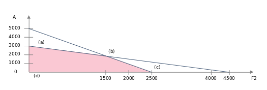
- Plot equality constraints. Determine which side of the graphs is the area of possible solutions. Shade it.
- Repeat Steps 1-3 for all restrictions

- Determine the scope (limited or unlimited) of possible solutions
- Solve constraint equations for all corner points of the graph. Determine the profit or profit margin in them (objective function).
- Replace inequalities with equalities
***
In our case, point b corresponds to the objective function, i.e. maximum margin profit
